Human in A.I. loop

September 9, 2016 Saurabh Bhatnagar12 Comments

A.I is out to get us. It will replace us all.. or maybe, it’s just another tool that we will get used to like calculators or iPhones.

fashion

If you are reading this post, chances are you are familiar with Artificial Intelligence, Deep Learning, Neural nets. I am not going to be pedantic and use them interchangeably.

If you don’t care for any of that, feel free to read this article as “Human in Machine Learning loop”. Or how to debug beyond metrics (smell a pattern in this blog?).

Let’s start with a practical example of something I built at Rent The Runway. RTR rents out high end designer dresses for a mass market price. We have a lot of folks who love us. And they are not shy about tagging us on their Instagram posts.

Wouldn’t it be great if we could show those Instagram photos on our product pages and help our customers find fashion inspiration through these high quality shots?

We already have photo reviews that our customers post on our site showing us how they wore it. It is a highly used feature for visitors. But customers have to submit to us directly for that to work.

My mind was set. It had to be done.

But how? While it is true that they tag #renttherunway or #myRTR, they don’t tag the exact dress name.

Obviously I brought a tank to a knife fight and built a convolutional neural net. This A.I that would look at these natural images and classify them as one of the thousands of dresses that we have currently on site. I named it DeepDress, but probably should have called it Dress2Vec… too late now. I used Torch to train and Benjamin’s waffle package to create an internal API that I can hit from any language. Since I have little patience, I used NVIDIA GPUs to speed up the training and tests.

I got all 30k Instagram posts at the time and I stored the metadata in Mongo (I know, I know but it’s great for unstructured).

Here is the code for that –

	import urllib.request
	import json
	from pymongo import MongoClient
	import time

	def fetchAndStash(url, client):
	try:
	response = urllib.request.urlopen(url + '&count=100')
	f = response.read()
	payload = f.decode('utf-8')
	j = json.loads(payload)

	if j['meta']['code'] == 200 : # Request worked
	for i in j['data']: # Loop through Instagram posts and save them
	try:
	# Hardcoded Database/Collection names.. change this
	result = client.DeepDress.InstagramV4.insert({'_id' : i['link'], 'payload' : i, 'image' : i['images']['low_resolution']['url']})
	except:
	print("bad batch url: " + url + '; tried to insert ' + i)
	with open('error', 'a') as of:
	of.write(f.decode('utf-8'))

	time.sleep(1) # Be nice
	fetchAndStash(j['pagination']['next_url'], client) # Follow the white rabbit

	else :
	print(url)
	except:
	print("Failed url ", url)

	def main():
	client = MongoClient()
	url = 'https://api.instagram.com/v1/tags/renttherunway/media/recent/?client_id=your_client_id_here'
	fetchAndStash(url, client) # could hit stack overflow.. but unlikely

	if __name__ == "__main__":
	main()

view raw

get_instagam.py

hosted with ❤ by GitHub

Then I looped through them and called my API to identify the dress and saved that.

	import urllib.request
	import json
	from pymongo import MongoClient
	import time
	from multiprocessing import Pool

	DEEP_DRESS_WGET = 'http://localhost/wget/?url='
	DEEP_DRESS_PREDICT = 'http://localhost/predict/'

	def wget_deep_dress(url):
	serviceurl = DEEP_DRESS_WGET + url
	response = urllib.request.urlopen(serviceurl)
	f = response.read()
	j = json.loads(f.decode('utf-8'))
	return(j['file_id'])

	def predict_deep_dress(file_id, top_n):
	serviceurl = DEEP_DRESS_PREDICT + '?file_id=' + file_id + '&top_n=' + top_n
	response = urllib.request.urlopen(serviceurl)
	f = response.read()
	j = json.loads(f.decode('utf-8'))
	return(j)


	client = MongoClient()
	db = client.DeepDress
	instagram = db.InstagramV4
	matches = db.MatchesV4
	# already tagged
	ids = set([m['_id'] for m in matches.find()])

	def match_and_save(i):
	try:
	if (i['_id'] not in ids):
	file_id = wget_deep_dress(i['image'])
	preds = predict_deep_dress(file_id, '3')
	result = matches.insert({'_id' : i['_id'], 'prediction' : preds})
	time.sleep(1) # Be nice
	return(1)
	except:
	return(0)


	pool = Pool(processes=5) # Don't make this too high – rate limits
	totals = pool.map(match_and_save, instagram.find())
	print(sum(totals), len(totals))

view raw

tag_deepdress.map.py

hosted with ❤ by GitHub

Mission accomplished and moving on.

Well my friends, if that were the case, I wouldn’t have written this post. So here is how a production system is really built.

One problem I knew ahead of time is that our inventory changes over time as we retire older styles and acquire new ones. DeepDress did not know of some very new dresses and none of the old ones. Old ones aren’t an issue since we wouldn’t want to display them anyway but there is a cold start problem that I hadn’t solved at the time.

Another issue is that I had trained the algorithm only on our dresses. While that is our bread and butter, we also rent bags, earrings, necklaces, bracelets, activewear, etc. I always start simple for v1. This means there were bound to be things classified incorrectly as the convnet sweats bullets trying to figure out which dress that Diane Von Furstenberg minaudiere looks like. We could use a lower bound on the probability of most likely class, but what should that threshold be?

Besides the above red flags, even if the identification were 100% accurate (ha), it would make sense to have someone in RTR verify that the image is in fact, fit for display on our site and consistent with our branding.

What we need to build is a gamified quick truther thingy that all our 200 employees in main office can log in during their lunch break and rate a few items. It better be interesting and fast because they have important things to do. It wouldn’t hurt to get verification of the same image from a few different folks so we build our confidence. Then there are nice to haves like responsive, reactive, and other fancy words that mean fun to use.

I could have built this in ruby or react or something that pleases my web developer friends. But I am a data scientist who is very familiar with R, so I built another shiny little thing in an hour. I am in good company. My friend Rajiv also loves understanding his A.I. creations in R.

Rough outline on what we want –

Start with a random seed for each session
Retrieve Instagram Images from that seed backwards
User has to choose one of N options
Upon choice, store the result back in Mongo
Automatically move on to the next one (shiny is responsive)
Every day, a job would restart the server, freezing what was done and starting on the next batch, moving back in time.

First we set up the global.R to get the relevant Instagram posts we will verify –

	library(mongolite)

	# Connections to mongo
	instagram <- mongo(collection = "InstagramV4", db = "DeepDress", url = "mongodb://localhost", verbose = FALSE)
	matches <- mongo(collection = "MatchesV4", db = "DeepDress", url = "mongodb://localhost", verbose = FALSE)
	corrections <- mongo(collection = "CorrectionsV4", db = "DeepDress", url = "mongodb://localhost", verbose = FALSE)

	# Get Instagram data we saved earlier
	ids.df <- instagram$find(fields = '{"_id" : 1, "payload.created_time" : 1}')
	ids.df.simple <- data.frame(id = ids.df$`_id`,
	created_time = ids.df$payload$created_time,
	stringsAsFactors = FALSE)

	# Reorder by newest
	ids.df.simple <- ids.df.simple[order(–as.numeric(ids.df.simple$created_time)), ]

	# What has already been corrected by users
	ids.done <- corrections$find(fields = '{"id" : 1}') # What has already been corrected

	# What's left
	ids.df.todo <- setdiff(ids.df.simple$id, ids.done$id)

view raw

reviews_truther_global.R

hosted with ❤ by GitHub

Then we create ui.R that my colleagues will see –

	library(shiny)

	shinyUI(fluidPage(

	# Application title
	titlePanel("Verify Auto-tagged dresses from Instagram"),

	# Sidebar with a slider input for number of bins
	sidebarLayout(
	sidebarPanel(
	textInput("email", "Your email", placeholder = "So that we can attribute the correction to you"),

	htmlOutput("instagram"),
	radioButtons("yesorno", "Accept tag?",
	c("Not a dress", "First", "Second", "Third", "None"), selected = "None"),
	actionButton("submit", "Submit"),
	helpText("Click the photo to see the original Instagram"),
	helpText("DeepDress AI might not know about some newer dresses. Esp dresses with <= 10 photo reviews"),
	helpText("The AI was written to match ANY PHOTO to our dresses. It does not know if what it is seeing is not a dress."),
	helpText("FAQ: Use 'Not a dress' if it is a Handbag, jacket, car or flower.. anything that's not a dress.")
	),

	# Show a plot of the generated distribution
	mainPanel(
	htmlOutput("deepDress"),
	hr(),
	h4("Match probability"),
	textOutput("deepDressProb")
	)
	)
	))

view raw

reviews_truther_ui.R

hosted with ❤ by GitHub

Finally we need to hook up some logic –

	shinyServer(function(input, output, session) {

	# Session level
	idx <- round(runif(1, 1, 2500)) # random place to start

	state <- reactive({
	if(input$submit > 0) { # Not on first page load
	isolate({ # Don't get reactive on me now
	answer <- input$yesorno

	m <- matches$find(query = paste0('{"_id": "', ids.df.todo[idx], '"}'), fields = '{}' ,limit = 1, pagesize=1)

	answer.clean <- ifelse(answer == "First",
	m$prediction$styleNames[[1]]$style[1],
	ifelse(answer == "Second",
	m$prediction$styleNames[[1]]$style[2],
	ifelse(answer == "Third",
	m$prediction$styleNames[[1]]$style[3],
	answer)))

	datum <- data.frame(email = input$email,
	id = ids.df.todo[idx],
	answer = answer.clean,
	ts = Sys.time()
	)
	corrections$insert(datum)
	})
	}
	idx <<- idx + 1 # Keep on moving
	})

	output$instagram <- renderPrint({
	state()
	i <- instagram$find(query = paste0('{"_id": "', ids.df.todo[idx], '"}'), fields = '{}' ,limit = 1, pagesize=1)
	cat(paste0("<a href='", i$`_id`,"' target='_blank'>",
	"<img src='", i$image, "' />",
	"</a>"))
	})

	getFirst <- reactive({
	state()
	m <- matches$find(query = paste0('{"_id": "', ids.df.todo[idx], '"}'), fields = '{}' ,limit = 1, pagesize=1)
	})

	output$deepDress <- renderPrint({
	m <- getFirst()
	cat(paste0("<img src='", m$prediction$styleNames[[1]]$urls$imageURL, "' />"))
	})

	output$deepDressProb <- renderText({
	m <- getFirst()
	paste(round(m$prediction$styleNames[[1]]$probability), '%')
	})

	})

view raw

reviews_truther_server.R

hosted with ❤ by GitHub

And shiny does the rest. Here is what this looks like in practice –

This slideshow requires JavaScript.

This was so successful that in the two weeks the POC was up, we had 3,281 verifications. Some colleagues (thanks Sam/Sandy) did as many as 350+ verifications over that time. It should be pointed out that besides an announcement email, there was no other push to do this.

We found that there were a significant number of posts that were not even dresses. I guess our fashionistas really love us. This is not a problem I knew about going into building this and was certainly not expecting high probability scores for the suggested class in some cases. It helped me fix it by adding a class for “not a dress” with actual training data (and noise).

Most importantly, we answered important questions like what this cute puppy wore.

puppy

And if that isn’t the most satisfying result, I don’t know what is.

We have some amazing employees (hi Sam/Liz/Amanda) who have can remember single dress on site. For mere mortals, matching a photo to something we have is nearly impossible.

DeepDress A.I toiled through all 30k photos and narrowing each down to 3 possible choices from our thousands. But it is humans who really save the day. As a result we have a golden database of Instagram photos mapped to exact product that took advantage of both their strengths. Look at that – humans and A.I can play together.

Hopefully this example demonstrates why it is useful to use your resources (company employees) to check your systems beyond the metrics before releasing things in the wild. I end up using shiny a lot for these sort of internal demos because I slice and dice the results in R. But do them in whatever you are comfortable in and aggressively re-evaluate those choices should they reach production. For example, we will rewrite the truther in Ruby now that it will be production to comply with our other standards. For demos, I have no emotional attachment to any language (close your ears C++).

I’m sure you guessed that could not have been the only reason I built DeepDress and you would be right. But today’s not a day to talk about that.

Matrix factorization

March 10, 2015March 10, 2015 Saurabh BhatnagarR, recommender, recommenderlab, Rstats14 Comments

Or fancy words that mean very simple things.

At the heart of most data mining, we are trying to represent complex things in a simple way. The simpler you can explain the phenomenon, the better you understand. It’s a little zen – compression is the same as understanding.

Warning: Some math ahead.. but stick with it, it’s worth it.

When faced with a matrix of very large number of users and items, we look to some classical ways to explain it. One favorite technique is Singular Value Decomposition, affectionately nicknamed SVD. This says that we can explain any matrix $A$ in the form

$A= USV^T$

Here

$A$ is of size num_users and num_products

$U$ is of size num_users and num_users

$S$ is a rectangular diagonal matrix of size num_users and num_products

$V$ is of size num_products and num_products

This is cool because the numbers in the diagonal $S$ are decreasing values of variance (roughly speaking). So the first number captures the most variance in $A$ , the second, less so, and so on, till all the numbers put together capture all the variance of $A$ .

You see where this is going. If we are comfortable with explaining only 10% of the variance, we can do so by only taking some of these values. We can then compress $A$ .

The other nice thing about all this is eigenvectors (which those roughly represent) are orthogonal. In other words, they are perpendicular to each other and there aren’t any mixed effects. If you don’t understand this paragraph, don’t worry. Keep on.

Consider that above can be rewritten as

$A = U\sqrt{S}\sqrt{S}V^T$

or –

$Y = X \Theta^T$

If $X$ is of size num_users and num_categories and $\Theta$ is of size num_products and num_categories, then we have a decent model that approximates $A$ into $Y$ . $Y$ is now called a low rank approximation of $A$ , or truncated SVD.

It is important to understand what these matrices represent. $X$ is the representation of users in some low dimension space (say romance, action). And $\Theta$ is the representation of products in the very same low dimension space. However, we don’t know exactly what these factors mean. They could be romance/action or they could NYC/Dallas. This is also why this method is sometimes called Latent Factor Matrix Factorization.. wow, quite a mouthful.

In my chapter in the book Data Mining Applications with R, I go over different themes of matrix factorization models (and other animals as well). But for now, I am only going to cover the basic one that works very well in practice. And yes, won the Netflix prize.

There is one problem with our formulation – SVD is only defined for dense matrices. And our matrix is usually sparse.. very sparse. Netflix’s challenge matrix was 1% dense, or 99% sparse. In my job at Rent the Runway, it is only 2% dense. So what will happen to our beautiful formula?

Machine learning is sort of a bastard science. We steal from beautiful formulations, complex biology, probability, Hoefding’s inequality, and derive rules of thumb from it. Or as an artist would say – get inspiration.

So here is what we are going to do. We are going to ignore all the null values when we solve this model. Our cost function now becomes

$J = R ( Y - X \Theta^T)^2 + \lambda (||X||^2 + ||\Theta||^2)$

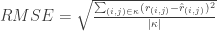
Here $Y - X\Theta^T$ is the difference between observed data and our prediction. $R$ is simply a matrix with 1 where we have a value and 0 where we do not. Multiplying these two we are only considering the cost when we observe a value. We are using L2 regularization of magnitude $\lambda$ . We are going to divide by 2 to make all other math easier. The cost is relative so it doesn’t matter.

$J = \frac{1}{2} R ( Y - X \Theta^T)^2 +\frac{1}{2} \lambda (||X||^2 + ||\Theta||^2)$

Using this our gradients become –

$\frac{\partial}{\partial{X}} = R (Y - X \Theta^T) \Theta + \lambda ||X||$

$\frac{\partial}{\partial{\Theta}} = R (Y - X \Theta^T)^T X+ \lambda ||\Theta||$

If we were wanted to minimize the cost function, we can move in the direction opposite to the gradient at each step, getting new estimates for $X$ and $\Theta$ each time.

This looks easy enough. One last thing. We now have what we want to minimize, but how do we do it? R provides many optimization tools. There is a whole CRAN page on it. For our purpose we will use out of the box optim() function. This allows us to access a fast optimization method L-BFGS-B. It’s not only fast, but also doesn’t take too memory intensive which is desirable in our case.

We need to give it the cost function and the gradient that we have above. It also expects one gradient function, so we need to unroll it out to do both our gradients.

	unroll_Vecs <- function (params, Y, R, num_users, num_movies, num_features) {
	# Unrolls vector into X and Theta
	# Also calculates difference between preduction and actual

	endIdx <- num_movies * num_features

	X <- matrix(params[1:endIdx], nrow = num_movies, ncol = num_features)
	Theta <- matrix(params[(endIdx + 1): (endIdx + (num_users * num_features))],
	nrow = num_users, ncol = num_features)

	Y_dash <- (((X %% t(Theta)) – Y) R) # Prediction error

	return(list(X = X, Theta = Theta, Y_dash = Y_dash))
	}

	J_cost <- function(params, Y, R, num_users, num_movies, num_features, lambda, alpha) {
	# Calculates the cost

	unrolled <- unroll_Vecs(params, Y, R, num_users, num_movies, num_features)
	X <- unrolled$X
	Theta <- unrolled$Theta
	Y_dash <- unrolled$Y_dash

	J <- .5 * sum( Y_dash ^2) + lambda/2 * sum(Theta^2) + lambda/2 * sum(X^2)

	return (J)
	}

	grr <- function(params, Y, R, num_users, num_movies, num_features, lambda, alpha) {
	# Calculates the gradient step
	# Here lambda is the regularization parameter
	# Alpha is the step size

	unrolled <- unroll_Vecs(params, Y, R, num_users, num_movies, num_features)
	X <- unrolled$X
	Theta <- unrolled$Theta
	Y_dash <- unrolled$Y_dash

	X_grad <- (( Y_dash %% Theta) + lambda X )
	Theta_grad <- (( t(Y_dash) %% X) + lambda Theta )

	grad = c(X_grad, Theta_grad)
	return(grad)
	}

	# Now that everything is set up, call optim
	print(
	res <- optim(par = c(runif(num_users * num_features), runif(num_movies * num_features)), # Random starting parameters
	fn = J_cost, gr = grr,
	Y=Y, R=R,
	num_users=num_users, num_movies=num_movies,num_features=num_features,
	lambda=lambda, alpha = alpha,
	method = "L-BFGS-B", control=list(maxit=maxit, trace=1))
	)

view raw

gistfile1.r

hosted with ❤ by GitHub

This is great, we can iterate a few times to approximate users and items into some small number of categories, then predict using that.

I have coded this into another package recommenderlabrats.

Let’s see how this does in practice against what we already have. I am going to use the same scheme as last post to evaluate these predictions against some general ones. I am not using Item Based Collaborative Filtering because it is very slow

	require(recommenderlab) # Install this if you don't have it already
	require(devtools) # Install this if you don't have this already
	# Get additional recommendation algorithms
	install_github("sanealytics", "recommenderlabrats")

	data(MovieLense) # Get data

	# Divvy it up
	scheme <- evaluationScheme(MovieLense, method = "split", train = .9,
	k = 1, given = 10, goodRating = 4)

	scheme

	# register recommender
	recommenderRegistry$set_entry(
	method="RSVD", dataType = "realRatingMatrix", fun=REAL_RSVD,
	description="Recommender based on Low Rank Matrix Factorization (real data).")

	# Some algorithms to test against
	algorithms <- list(
	"random items" = list(name="RANDOM", param=list(normalize = "Z-score")),
	"popular items" = list(name="POPULAR", param=list(normalize = "Z-score")),
	"user-based CF" = list(name="UBCF", param=list(normalize = "Z-score",
	method="Cosine",
	nn=50, minRating=3)),
	"Matrix Factorization" = list(name="RSVD", param=list(categories = 10,
	lambda = 10,
	maxit = 100))
	)

	# run algorithms, predict next n movies
	results <- evaluate(scheme, algorithms, n=c(1, 3, 5, 10, 15, 20))

	# Draw ROC curve
	plot(results, annotate = 1:4, legend="topleft")

	# See precision / recall
	plot(results, "prec/rec", annotate=3)

view raw

recommenderlab-test RSVD

hosted with ❤ by GitHub

It does pretty well. It does better than POPULAR and is equivalent to UBCF. So why use this over UBCF or the other way round?

This is where things get interesting. This algorithm can be sped up quite a lot and more importantly, parallelised. It uses way less memory than UBCF and is more scalable.

Also, if you have already calculated $\Theta$ , i.e. your items in some lower dimensional space, you might get away with just putting the users in that space. Now things become really fast because all you have to do is keep $\Theta$ fixed and figure out $X$ .

I have gone ahead and implemented a version where we just calculate $\Theta$ , I leave it to you as an exercise to modify the code above to test this out as well. The algorithm is called RSVD_SPLIT. Also feel free to try other values of categories, lambda and maxit and see how things change.

On the other hand, the latent categories are very hard to explain. For UBCF you can say this user is similar to these other users. For IBCF, one can say this item that the user picked is similar to these other items. But that not the case for this particular flavor of matrix factorization. We will re-evaluate these limitations later.

The hardest part for a data scientist is to disassociate themselves from their dear models and watch them objectively in the wild. Our simulations and metrics are always imperfect but necessary to optimize. You might see your favorite model crash and burn. And a lot of times simple linear regression will be king. The job is to objectively measure them, tune them and see which one performs better in your scenario.

Good luck.

Testing recommender systems in R

June 10, 2012June 12, 2012 Saurabh BhatnagarR, recommender, recommenderlab, Rstats9 Comments

Recommender systems are pervasive. You have encountered them while buying a book on barnesandnoble, renting a movie on Netflix, listening to music on Pandora, to finding the bar visit (FourSquare). Saar for Revolution Analytics, had demonstrated how to get started with some techniques for R here.

We will build some using Michael Hahsler’s excellent package – recommenderlab. But to build something we have to learn to recognize when it is good. For this reason we will talk about some metrics quickly –

– RMSE (Root Mean Squared Error) : Here we measure far were real ratings from the ones we predicted. Mathematically, we can write it out as

$RMSE = \sqrt\frac{\sum_{(i,j) \in \kappa}(r_{(i,j)} - \hat {r}_{(i,j)})^2}{|\kappa|}$

where $\kappa$ is the set of all user-item pairings $(i, j)$ for which we have a predicted rating $\hat r_{(i,j)}$ and a known rating $r_{(i,j)}$ which was not used to learn the recommendation model.

Here at sane.a.lytics, I will talk about when an analysis makes sense and when it doesn’t. RMSE is a great metric if you are measuring how good your predicted ratings are. But if you want to know how many people clicked on your recommendation, I have a different metric for you.

– Precision/Recall/f-value/AUC: Precision tells us how good the predictions are. In other words, how many were a hit.

Recall tells us how many of the hits were accounted for, or the coverage of the desirable outcome.

Precision and recall usually have an inverse relationship. This becomes an even bigger issue for rare issue phenomenon like recommendations. To tackle this problem, we will use f-value. This is nothing but the harmonic mean of precision and recall.

Another popular measure is AUC. This is roughly analogous. We will go ahead and use this for now for our comparisons of recommendation effectiveness.

– ARHR (Hit Rate): Karypis likes this metric.

$ARHR = \frac{1}{\#users} \sum_{i=1}^{\#hits} \frac{1}{p_i}$

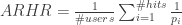
where $p$ is the position of the item in a ranked list.

OK, on to the fun stuff.

They are a few different ways to build a recommender system

Collaborative Filtering : If my friend Jimmy tells me that he liked the movie “Drive”, I might like it too since we have similar tastes. However if Paula tells me she liked “The Notebook”, I might avoid it. This is called UBCF (User-based collaborative filtering). Another way to think about it is that this is soft-clustering. We find Users with similar tastes (neighbourhood) and use their preferences to build yours.

Another flavour of this is IBCF (Item Based Collaborative Filtering). If I watched “Darjeeling Limited”, I might be inclined to watch “The Royal Tannenbaums” but not necessarily “Die Hard”. This is because the first two are more similar in the users who have watched/rated them. This is a rather simple to compute as all we need is the covariance between products to find out what this might be.

Let’s compare both approaches on some real data (thanks R)

	# Load required library
	library(recommenderlab) # package being evaluated
	library(ggplot2) # For plots

	# Load the data we are going to work with
	data(MovieLense)
	MovieLense
	# 943 x 1664 rating matrix of class ‘realRatingMatrix’ with 99392 ratings.

	# Visualizing a sample of this
	image(sample(MovieLense, 500), main = "Raw ratings")

view raw

recommenderlab-1-1.R

hosted with ❤ by GitHub

	# Visualizing ratings
	qplot(getRatings(MovieLense), binwidth = 1,
	main = "Histogram of ratings", xlab = "Rating")
	summary(getRatings(MovieLense)) # Skewed to the right
	# Min. 1st Qu. Median Mean 3rd Qu. Max.
	# 1.00 3.00 4.00 3.53 4.00 5.00

view raw

recommenderlab-1-2.R

hosted with ❤ by GitHub

	# How about after normalization?
	qplot(getRatings(normalize(MovieLense, method = "Z-score")),
	main = "Histogram of normalized ratings", xlab = "Rating")
	summary(getRatings(normalize(MovieLense, method = "Z-score"))) # seems better
	# Min. 1st Qu. Median Mean 3rd Qu. Max.
	# -4.8520 -0.6466 0.1084 0.0000 0.7506 4.1280

view raw

recommenderlab-1-3.R

hosted with ❤ by GitHub

	# How many movies did people rate on average
	qplot(rowCounts(MovieLense), binwidth = 10,
	main = "Movies Rated on average",
	xlab = "# of users",
	ylab = "# of movies rated")
	# Seems people get tired of rating movies at a logarithmic pace. But most rate some.

view raw

recommenderlab-1-4.R

hosted with ❤ by GitHub

	# What is the mean rating of each movie
	qplot(colMeans(MovieLense), binwidth = .1,
	main = "Mean rating of Movies",
	xlab = "Rating",
	ylab = "# of movies")

	# The big spike on 1 suggests that this could also be intepreted as binary
	# In other words, some people don't want to see certain movies at all.
	# Same on 5 and on 3.
	# We will give it the binary treatment later

view raw

recommenderlab-1-5.R

hosted with ❤ by GitHub

	recommenderRegistry$get_entries(dataType = "realRatingMatrix")
	# We have a few options

	# Let's check some algorithms against each other
	scheme <- evaluationScheme(MovieLense, method = "split", train = .9,
	k = 1, given = 10, goodRating = 4)

	scheme

	algorithms <- list(
	"random items" = list(name="RANDOM", param=list(normalize = "Z-score")),
	"popular items" = list(name="POPULAR", param=list(normalize = "Z-score")),
	"user-based CF" = list(name="UBCF", param=list(normalize = "Z-score",
	method="Cosine",
	nn=50, minRating=3)),
	"item-based CF" = list(name="IBCF2", param=list(normalize = "Z-score"
	))

	)

	# run algorithms, predict next n movies
	results <- evaluate(scheme, algorithms, n=c(1, 3, 5, 10, 15, 20))

	# Draw ROC curve
	plot(results, annotate = 1:4, legend="topleft")

	# See precision / recall
	plot(results, "prec/rec", annotate=3)

view raw

recommenderlab-1-6.R

hosted with ❤ by GitHub

It seems like UBCF did better than IBCF. Then why would you use IBCF? The answer lies is when and how are you generating recommendations. UBCF saves the whole matrix and then generates the recommendation at predict by finding the closest user. IBCF saves only k closest items in the matrix and doesn’t have to save everything. It is pre-calculated and predict simply reads off the closest items.

Predictably, RANDOM is the worst but perhaps surprisingly it seems, its hard to beat POPULAR. I guess we are not so different, you and I.

In the next post I will go over some other algorithms that are out there and how to use them in R. I would also recommend reading Michael’s documentation on recommenderlab for more details.

Also added this to r-bloggers. Please check it out for more R goodies.

Share this:

Like this:

Share this:

Like this:

Share this:

Like this: