
Or fancy words that mean very simple things.
At the heart of most data mining, we are trying to represent complex things in a simple way. The simpler you can explain the phenomenon, the better you understand. It’s a little zen – compression is the same as understanding.
Warning: Some math ahead.. but stick with it, it’s worth it.
When faced with a matrix of very large number of users and items, we look to some classical ways to explain it. One favorite technique is Singular Value Decomposition, affectionately nicknamed SVD. This says that we can explain any matrix 

Here


This is cool because the numbers in the diagonal
You see where this is going. If we are comfortable with explaining only 10% of the variance, we can do so by only taking some of these values. We can then compress
The other nice thing about all this is eigenvectors (which those roughly represent) are orthogonal. In other words, they are perpendicular to each other and there aren’t any mixed effects. If you don’t understand this paragraph, don’t worry. Keep on.
Consider that above can be rewritten as

or –

If 


It is important to understand what these matrices represent.
In my chapter in the book Data Mining Applications with R, I go over different themes of matrix factorization models (and other animals as well). But for now, I am only going to cover the basic one that works very well in practice. And yes, won the Netflix prize.
There is one problem with our formulation – SVD is only defined for dense matrices. And our matrix is usually sparse.. very sparse. Netflix’s challenge matrix was 1% dense, or 99% sparse. In my job at Rent the Runway, it is only 2% dense. So what will happen to our beautiful formula?
Machine learning is sort of a bastard science. We steal from beautiful formulations, complex biology, probability, Hoefding’s inequality, and derive rules of thumb from it. Or as an artist would say – get inspiration.
So here is what we are going to do. We are going to ignore all the null values when we solve this model. Our cost function now becomes

Here 


Using this our gradients become –


If we were wanted to minimize the cost function, we can move in the direction opposite to the gradient at each step, getting new estimates for
This looks easy enough. One last thing. We now have what we want to minimize, but how do we do it? R provides many optimization tools. There is a whole CRAN page on it. For our purpose we will use out of the box optim() function. This allows us to access a fast optimization method L-BFGS-B. It’s not only fast, but also doesn’t take too memory intensive which is desirable in our case.
We need to give it the cost function and the gradient that we have above. It also expects one gradient function, so we need to unroll it out to do both our gradients.
This file contains hidden or bidirectional Unicode text that may be interpreted or compiled differently than what appears below. To review, open the file in an editor that reveals hidden Unicode characters.
Learn more about bidirectional Unicode characters
| unroll_Vecs <- function (params, Y, R, num_users, num_movies, num_features) { | |
| # Unrolls vector into X and Theta | |
| # Also calculates difference between preduction and actual | |
| endIdx <- num_movies * num_features | |
| X <- matrix(params[1:endIdx], nrow = num_movies, ncol = num_features) | |
| Theta <- matrix(params[(endIdx + 1): (endIdx + (num_users * num_features))], | |
| nrow = num_users, ncol = num_features) | |
| Y_dash <- (((X %*% t(Theta)) – Y) * R) # Prediction error | |
| return(list(X = X, Theta = Theta, Y_dash = Y_dash)) | |
| } | |
| J_cost <- function(params, Y, R, num_users, num_movies, num_features, lambda, alpha) { | |
| # Calculates the cost | |
| unrolled <- unroll_Vecs(params, Y, R, num_users, num_movies, num_features) | |
| X <- unrolled$X | |
| Theta <- unrolled$Theta | |
| Y_dash <- unrolled$Y_dash | |
| J <- .5 * sum( Y_dash ^2) + lambda/2 * sum(Theta^2) + lambda/2 * sum(X^2) | |
| return (J) | |
| } | |
| grr <- function(params, Y, R, num_users, num_movies, num_features, lambda, alpha) { | |
| # Calculates the gradient step | |
| # Here lambda is the regularization parameter | |
| # Alpha is the step size | |
| unrolled <- unroll_Vecs(params, Y, R, num_users, num_movies, num_features) | |
| X <- unrolled$X | |
| Theta <- unrolled$Theta | |
| Y_dash <- unrolled$Y_dash | |
| X_grad <- (( Y_dash %*% Theta) + lambda * X ) | |
| Theta_grad <- (( t(Y_dash) %*% X) + lambda * Theta ) | |
| grad = c(X_grad, Theta_grad) | |
| return(grad) | |
| } | |
| # Now that everything is set up, call optim | |
| print( | |
| res <- optim(par = c(runif(num_users * num_features), runif(num_movies * num_features)), # Random starting parameters | |
| fn = J_cost, gr = grr, | |
| Y=Y, R=R, | |
| num_users=num_users, num_movies=num_movies,num_features=num_features, | |
| lambda=lambda, alpha = alpha, | |
| method = "L-BFGS-B", control=list(maxit=maxit, trace=1)) | |
| ) |
This is great, we can iterate a few times to approximate users and items into some small number of categories, then predict using that.
I have coded this into another package recommenderlabrats.
Let’s see how this does in practice against what we already have. I am going to use the same scheme as last post to evaluate these predictions against some general ones. I am not using Item Based Collaborative Filtering because it is very slow
This file contains hidden or bidirectional Unicode text that may be interpreted or compiled differently than what appears below. To review, open the file in an editor that reveals hidden Unicode characters.
Learn more about bidirectional Unicode characters
| require(recommenderlab) # Install this if you don't have it already | |
| require(devtools) # Install this if you don't have this already | |
| # Get additional recommendation algorithms | |
| install_github("sanealytics", "recommenderlabrats") | |
| data(MovieLense) # Get data | |
| # Divvy it up | |
| scheme <- evaluationScheme(MovieLense, method = "split", train = .9, | |
| k = 1, given = 10, goodRating = 4) | |
| scheme | |
| # register recommender | |
| recommenderRegistry$set_entry( | |
| method="RSVD", dataType = "realRatingMatrix", fun=REAL_RSVD, | |
| description="Recommender based on Low Rank Matrix Factorization (real data).") | |
| # Some algorithms to test against | |
| algorithms <- list( | |
| "random items" = list(name="RANDOM", param=list(normalize = "Z-score")), | |
| "popular items" = list(name="POPULAR", param=list(normalize = "Z-score")), | |
| "user-based CF" = list(name="UBCF", param=list(normalize = "Z-score", | |
| method="Cosine", | |
| nn=50, minRating=3)), | |
| "Matrix Factorization" = list(name="RSVD", param=list(categories = 10, | |
| lambda = 10, | |
| maxit = 100)) | |
| ) | |
| # run algorithms, predict next n movies | |
| results <- evaluate(scheme, algorithms, n=c(1, 3, 5, 10, 15, 20)) | |
| # Draw ROC curve | |
| plot(results, annotate = 1:4, legend="topleft") | |
| # See precision / recall | |
| plot(results, "prec/rec", annotate=3) |
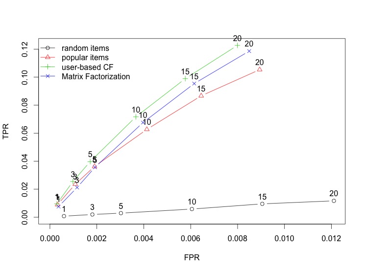

It does pretty well. It does better than POPULAR and is equivalent to UBCF. So why use this over UBCF or the other way round?
This is where things get interesting. This algorithm can be sped up quite a lot and more importantly, parallelised. It uses way less memory than UBCF and is more scalable.
Also, if you have already calculated
I have gone ahead and implemented a version where we just calculate
On the other hand, the latent categories are very hard to explain. For UBCF you can say this user is similar to these other users. For IBCF, one can say this item that the user picked is similar to these other items. But that not the case for this particular flavor of matrix factorization. We will re-evaluate these limitations later.
The hardest part for a data scientist is to disassociate themselves from their dear models and watch them objectively in the wild. Our simulations and metrics are always imperfect but necessary to optimize. You might see your favorite model crash and burn. And a lot of times simple linear regression will be king. The job is to objectively measure them, tune them and see which one performs better in your scenario.
Good luck.

Hi: I read your example about matrix factorization in R and it was interesting. Thanks for it. Just a couple of things.
A) I wouldn’t use L-BFGS-B because it can be extremely buggy. See this URL for details. http://www.ece.northwestern.edu/~morales/PSfiles/acm-remark.pdf. I currently use Rvmmin as a replacement. It is a work in progess but seems to be bug free and solid and fast and reliable.
B) What is the size of your initial movie matrix ? I didn’t and don’t currentyl have time to play with your example but I played around with matrix factorization in R a couple of years ago and most of the algorithms I tried ending up choking because the movieLens matrix was too large. What is the size of one were you using in your example ? Maybe using it inside Recommenderlab helps with the size issue. I didn’t use Recommenderlab when I played around a few years ago. Thanks for any clarifications.
Mark
Hi Mark,
Thanks for your response.
A) I was not familiar with this result. It looks like they achieved an improvement in speed.. which is very appreciated. I will try out Rvmmin.
B) MovieLense dataset that comes with recommenderlab is 943 users and 1663 movies with only 99,392 ratings. It occupies 1.3Mb. The reduction is due to the use of Matrix library that has some nice sparse Matrix classes.
Having said that, in this particular implementation of the algorithm, I simply used regular matrices to mock this up. A regular matrix of that size takes 12Mb. It can easily be rewritten to use the sparse matrix class but there is a small performance penalty.
The above results ran 100 iterations on my 8GB, 3 year old Macbook Pro in 26 seconds.
This algorithm does not require much more memory and search space if your number of categories is small (small matrices). But you will need roughly 2.5X the size of your initial matrix.
To give perspective, I have run a version of this algorithm on large AWS servers with 300k users and 2,500 products and it runs 300 iterations in under 4 hours. I might do another post on tips on speeding this sort of thing and having a smaller footprint.
I don’t understand. If Y= X Theta’ then the first term in J, R(Y-X Theta’)^2, should always be zero. Do you mean R(A-X Theta’)^2?
Nevermind. When we don’t know X and Theta, then we have to find an approximation for each, subject to some cost function. Got it.
Thanks Saurabhat for your responses.
1) Note that the L-BFGS-B problem is NOT JUST AN ISSUE OF SPEED. There are SERIOUS problems with L-BFGS-B. I’ve tested it
a lot in a different problem context and it can often terminate early because of the precision issue. ( i.e: terminate when the gradients
on the inactive constraints are not zero ). So, you can get estimates that are claimed to be optimal that actually aren’t.
2) If I memory serves me correctly, there are a couple of different movieLens data sets. It sounds like you are using the one which
is relatively small. If you go up in size ( I think the medium sized one is the one I used ), you will probably run into problems in R.
3) I don’t have time at the moment but when I get some, if you like, I can send you some R code that illustrates the problem in 2). Maybe you can improve on what I did by using tricks in R. I didn’t know that many so I eventually tried to write a different algorithm for solving the
matrix factorization problem. Then, while I was working on that, Hastie and Tibishrani and whoever works with them sent a package to CRAN for solving matrix factorization problems. I stopped what I was doing because I was realistic and knew that whatever I was working on couldn’t be an improvement to what they did. I moved on and didn’t look into what they did but, knowing them, I’m confident it can probably be used to deal with the issue in 2).
All the best and thanks for the interesting post. Email me if you’re interested in the R matrix factorization code that illustrates the issue in 2). I can dig it up. Background is that I was taking Andrew Ng’s course and then started pursuing matrix factorization further in R but, as I described, eventually hit a wall.
Mark
[…] Matrix Factorization At the heart of most data mining, we are trying to represent complex things in a simple way. The simpler you can explain the phenomenon, the better you understand. It’s a little zen – compression is the same as understanding. Warning: Some math ahead.. but stick with it, it’s worth it. […]
Hi Saurabh: I did a little bit of digging and did manage to retrieve my last attempt at using R functions to solve a fairly large matrix factorization problem. I have the data set and the R code but I don’t think it can be attached here and I couldn’t find your direct email address.
Unfortunately, I never made it into a package but I think you can follow it pretty easily if you’re interested. It’s probably very similar to what you did in the R example in your blog. Also, what I
said about L-BFGS-B is correct but then algorithm I was using instead of L-BFGS-B was Rcgmin rather than Rvmmin. ( I use Rvmmin but for something else ). Rcgmin was the best algorithmI could find and it took 4 hours to solve the matrix factorization problem that I was dealing with. But that was waaay better than evetything else because everything else never even got to a solution.
Anyway, if you want the R code, let me know at markleeds2@gmail.com. With your knowledge of
the Matrix package, maybe there’s a way to make it even faster. I’d be interested in collaborating
on this at some point because it always bothered me that I was never able to carry the project
through to get a more reasonable timing. All the best.
Mark
Thanks Mark.. I’m curious. Emailing you.
I changed the code to take in any optimization method as a parameter (as long as it takes a cost and a gradient function). I then tested Rcgmin and it seems to work fine. I did not see a major difference in results (or timing) between that and out of the box optim for my data.
Having said that, please feel free to use your own optimization method. Just pass it in.
Here is a gist of my test –
This file contains hidden or bidirectional Unicode text that may be interpreted or compiled differently than what appears below. To review, open the file in an editor that reveals hidden Unicode characters.
Learn more about bidirectional Unicode characters
Rcgmin test
hosted with ❤ by GitHub
This works nicely in practice. I am able to use this on a sample of Rent The Runway data (350k users x 3k users) and am able to do 300 iterations of that in 3 hours. I use some tricks to speed R up that I will detail in a follow up post.
Hi Saurabh,
I was just trying to install the recommenderlabrats to play around with. I am really curious about your approach and how it will perform. However, I constantly get this error when I try to install via devtools:
“Downloading github repo recommenderlabrats/sanealytics@master
Error in download(dest, src, auth) : client error: (404) Not Found”
Can you check your github? 🙂
Thanks in advance. I can’t wait to play around with those variations of Matrix Factorization. I programmed one myself and am curious to check your performance.
I’m not sure what could have been wrong. It works for me.. can you give it a try again?
Hey, that method is deprecated, you have to use: install_github(“sanealytics/recommenderlabrats”)
Hi Saurabh,
Thanks for the article. I am trying to figure out how recommenderlabrats work, got to your github, but cannot seem to be able to install the package. Could you please have a quick look at my error message? Perhaps I am missing something —
installing to /Library/Frameworks/R.framework/Versions/3.2/Resources/library/recommenderlabrats/libs
** R
** preparing package for lazy loading
Warning: package ‘recommenderlab’ was built under R version 3.2.5
Warning: package ‘arules’ was built under R version 3.2.5
Warning: package ‘proxy’ was built under R version 3.2.5
Warning: package ‘RcppArmadillo’ was built under R version 3.2.5
Error : Entry already in registry.
Error : unable to load R code in package ‘recommenderlabrats’
ERROR: lazy loading failed for package ‘recommenderlabrats’
* removing ‘/Library/Frameworks/R.framework/Versions/3.2/Resources/library/recommenderlabrats’
Error: Command failed (1)
Sorry to hear that. Can you open an issue in the git repo? Let’s tackle it there.
[…] you need a refresher on Matrix Factorization, please see this old post. Now come back to this and let’s talk about a really important addition -> Implicit […]