This is second post in the series started here. The goal of this experiment is to help new data scientists see how things are really built outside textbooks and kaggle. Also, if you want to work on challenging real world problems (not ads), come work with us.
The previous post covered proposals with Engineering because data science can’t stand without their shoulders. There is no mention of the model. This is intentional. Before you build anything, it is important to establish what success looks like. Data science classes have it all backwards, that you are given clean pertinent data and the metric, and you can just apply your favorite model. Real life is messy.
So let’s talk about what is our success metric for Data Science Track.
When an Unlimited customer is ready to swap out for a set of new dresses, she comes to our site and browses. This is a long cycle where she will try a lot of different filters and pathways to narrow down the products she wants. These products are filtered by availability at the time. We are not a traditional e-commerce site and are out of some dresses at any given point. If we don’t have a barcode in her size, we won’t display it that day. This is controlled by a home-grown complicated state machine software called reservation calendar. Think hotel bookings.
We can’t control what will be available the day she comes back. So there are a few metrics that might matter:
- PICKS: Does she pick the dress that was recommended?
- SESSION_TIME: Does it take her less time to get to the dress? Is the visit shorter?
- HEARTS: Did she favorite the dress. So even though she won’t pick it this time, she likes it and could rent it later.
I like PICKS because it is the most honest indicator of whether she was content. However availability skews it – she might have picked that dress if it were available that day.
SESSION_TIME is interesting because while this is a great theory, nothing shows conclusively that spending less time on site reduces churn. If anything, we see the opposite. This is because an engaged user might click around more and actually stay on the site longer. Since I don’t understand all these dynamics, I’m not going to check this now.
HEARTS is a good proxy. However it is possible that she might favorite things because they are pretty but not pick them. This was the case at Barnes & Nobles where I pulled some Facebook graph data and found little correlation with authors people actually bought. However, we have done a lot of analysis where for Unlimited users, this correlates with picks very nicely. So Unlimited users are actually using hearts as their checkout mechanism.
We also have shortlists, but all shortlists are hearts so we can just focus on hearts for now.
OK, so we all agreed that HEARTS is the metric we will tune against. Of course, PICKS needs to be monitored but this is the metric we will chase for now.
Now that we have the metric, let’s talk data.
We have:
- membership information
- picks (orders)
- classic orders
- product views
- hearts
- shortlists
- searches and other clicks
- user profile – size, etc
- reviews
- returns
- Try to buy data
For a new data scientist, this would be the most frustrating part. Each data has it’s own quirks and learnings. It takes time to understand all those. Luckily, we are familiar with these.
Baseline Models
We want a baseline model. And ideally, more than one model so we can compare against this baseline and see where we are.
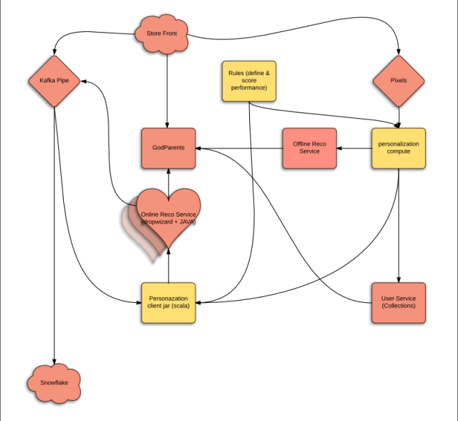
Current recommendations are running on a home grown Bayesian platform (written in scala). For classic recommendations, they are calculating :
P(s | u) = P(e | u) * P(s | e)
where s = style (product). u = user, e = event.
In other words, it estimates the probability of user liking a style based on user going to an event. We use shortlists, product views and other metadata to estimate these.
Since we have this pipeline already, the path of least resistance would be to do something like
P(s | u) = P(c | u) * P(s | c)
where c is a carousel. And we can basically keep the same math and calculations.
But what are these carousels?
There are global carousels, user carousels based on some products (like product X) and attribute based.
An attribute carousel is something like ‘dresses for a semi-formal wedding’. We have coded these as formalities (subjective but lot of agreement). They could be tops with spring seasonality, etc.
OK, but this poses a problem. The above model is using a Dirichlet to calculate all this and there is an assumption that different carousels are independent.
Is this a problem? We won’t know till we build it. And the path to build this is fast.
What else can we do?
When I joined RTR 4+ years ago, the warehouse was in MySQL and all click logs were in large files on disk. To roll out the first reco engine, I created our current Data Warehouse, Vertica which is a Massively Parallel Processing RDBMS. Think Hadoop but actually made for queries. This allowed me to put the logs in there, join to orders, etc. I could talk about my man crush on Turing aware winner, Michael Stonebraker but this is not the time to geek out about databases.
Importantly, it also allows R extensions to run on each node. So besides bringing the data warehouse to the 21st century, I used that to create recommendations that run where the data is. This is how we did recommendations till two years ago when we switched to the Bayesian model I described above.
I used Matrix Factorization Methods that I have described before. The best one was Implicit where we don’t use ratings but rather implicit assumption that anything picked is the same. This aligns nicely with our problem. So my plan was to try it with this data.
My old production code is long gone but I still have what I used for testing here. It’s written in Rcpp (C++ with R bindings) and performs fairly well. It does not use sparse matrices (commit pending feature request in base library). We have to rewrite this in scala anyway so that might be the time to scale this out (batch gradient descent and other tricks). But we can run it right now and use this algorithm to see if it’s worth the effort.
This bears repeating, Implicit Matrix Factorization or SVD++ is the model you want to baseline against if you are new to this. DO NOT USE cosine distances on your user x product matrices. That won’t scale.
AI
Three years ago, I also started working on AI (like everyone). But mostly because I realized that our product is visual. And we could only go so far with stylist tagged attributes. This led to a few products, which are collectively called DeepDress AI internally. The most outward facing is this Chrome extension that will let you rent a dress on any e-retailer’s page. There are also lesser features like visual search via App, product to product recommendations. The most creative is a tool used by the Buying team to check which products match the ones they are considering, and how did they do in the past?
I obviously want to leverage that research here. However it won’t be the baseline. It will be the next model we try.
Carousels go round and round
For both algorithms, we first need to get more clarity on carousels. Sean built an internal visualizer using R/Shiny and we asked our buyers and fashion teams to rate a product in 8 classes -> minimalist, romantic, glamorous, sexy, edgy, boho, preppy, casual. No explanations were given but that team is highly sophisticated and has a very good view of this taxonomy.
One view is that these merchandising tags along with formality tags (from 1-apparel to 10-ballgowns) would form the first set of carousels.
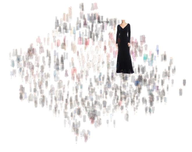
My contention is that if we use SVD++ or AI, the latent space should be explainable since the product is visual. However there is a risk we won’t be able to find meaningful things within the timeframe.
So we broke this problem down into two sections:
- Sean to verify the validity of these style tags. And collect more by working with other teams.
- I will try to predict these style tags using AI (ideally DeepDress). Time is of the essence. If I can prove this out, Sean does not have to ask the other teams.
- Once Matrix Factorization is done, I will explore to see if I can find meaningful things there
I had started looking to predict these style tags five days before we started the project. But couldn’t finished it. I tried to spend an evening after work looking to see if there is something there.
style personas
When buyers log into Sean’s sytem, they get a product and have to rate all eight style personas between 1 and 8. Once a style gets 10 ratings, it is not shown again.
So while Sean is embarking on finding out of 10 ratings have agreement, I started to predict them via looking at the dress itself and nothing more.
This is a throwaway model. Even if it works, it just proves that DeepDress captures the essence of these style persona attributes and we can use AI directly. So I have to timebox it.
At this point, there are only 1418 styles that have been completed. I received the medians of these ratings for 60% of the data, 851 styles. This is what the data looks like –
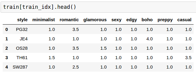
out of which 32 are all 1s.
So I have only 819 examples where we don’t always have a clear dominant class. I further divided that into my own train/validation styles with 80/20 split. At the end I have only 645 styles I am training on.
This would normally be hopeless. But one trick is to take a network trained a larger dataset and perturb the weights by very little. This is called finetuning in literature.
I could have fine-tuned DeepDress but instead I started by fine-tuning Vgg11 to get going quickly.
The model looks like this –
FineTuneModel (
  (features): DataParallel (
    (module): Sequential (
      (0): Conv2d(3, 64, kernel_size=(3, 3), stride=(1, 1), padding=(1, 1))
      (1): ReLU (inplace)
      (2): MaxPool2d (size=(2, 2), stride=(2, 2), dilation=(1, 1))
      (3): Conv2d(64, 128, kernel_size=(3, 3), stride=(1, 1), padding=(1, 1))
      (4): ReLU (inplace)
      (5): MaxPool2d (size=(2, 2), stride=(2, 2), dilation=(1, 1))
      (6): Conv2d(128, 256, kernel_size=(3, 3), stride=(1, 1), padding=(1, 1))
      (7): ReLU (inplace)
      (8): Conv2d(256, 256, kernel_size=(3, 3), stride=(1, 1), padding=(1, 1))
      (9): ReLU (inplace)
      (10): MaxPool2d (size=(2, 2), stride=(2, 2), dilation=(1, 1))
      (11): Conv2d(256, 512, kernel_size=(3, 3), stride=(1, 1), padding=(1, 1))
      (12): ReLU (inplace)
      (13): Conv2d(512, 512, kernel_size=(3, 3), stride=(1, 1), padding=(1, 1))
      (14): ReLU (inplace)
      (15): MaxPool2d (size=(2, 2), stride=(2, 2), dilation=(1, 1))
      (16): Conv2d(512, 512, kernel_size=(3, 3), stride=(1, 1), padding=(1, 1))
      (17): ReLU (inplace)
      (18): Conv2d(512, 512, kernel_size=(3, 3), stride=(1, 1), padding=(1, 1))
      (19): ReLU (inplace)
      (20): MaxPool2d (size=(2, 2), stride=(2, 2), dilation=(1, 1))
    )
  )
  (fc): Sequential (
    (0): Linear (25088 -> 4096)
    (1): ReLU (inplace)
    (2): Dropout (p = 0.5)
    (3): Linear (4096 -> 4096)
    (4): ReLU (inplace)
    (5): Dropout (p = 0.5)
  )
  (classifier): Sequential (
    (0): Linear (4096 -> 8)
  )
)
I decided on minimizing KL-divergence which meant the last layer should do log_softmax(). It also means I normalized the input by subtracting 1 and dividing by the sum of the row to make things add up to 1, a valid probability distribution.
To train this, all rows are frozen except last one for first 100 epochs. It also reduced the learning rate every now and then.
I then went to sleep and the model churn away on my tiny laptop with a small GPU.
I woke up to these long loss curves
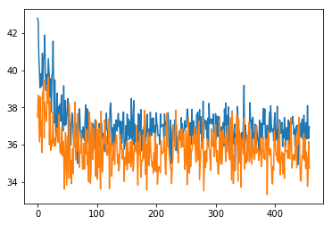
where orange line is train loss and blue is validation loss. They are so jarry because of dropout, random modifications to training images, I’ve tuned them for too long and really, too little data. I could spend more time debugging but won’t for now.
I also calculated accuracy as comparing the highest probable class. If there are two, I took the first one. So if the highest probability was for minimalist, then I was checking to make sure that the highest in predictions is also the same. TOP1 accuracy was then around 40%
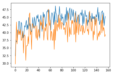
(zoomed in TOP1 accuracy)
I also calculated TOP2 accuracy that comes out to be 60%.
I chose the model at an epoch with highest TOP2 accuracy in validation set.
Here, per class TOP1 accuracy in my own validation set comes out to be –
Accuracy of minimalist : 25 %
Accuracy of romantic : 75 %
Accuracy of glamorous : 31 %
Accuracy of  sexy : 25 %
Accuracy of  edgy : 25 %
Accuracy of  boho : 68 %
Accuracy of preppy : 43 %
Accuracy of casual : 37 %
Did we overfit? Are these terrible results? I don’t know yet but I am not running a GAN for this.
Here is the code in pytorch, in case anyone has a similar problem: Finetune to minimize KL-divergence.
Wait till tomorrow to know how this works out as well as other experiments.
PS. Featured image via Mahbubur Rahman
PPS. Does the above sound interesting? Come work with us