Cross posting to original article posted here
Uncategorized
How I scaled Machine Learning to a Billion dollars: Strategy
Cross posting here to original article I posted in https://medium.com/@analyticsaurabh/how-i-scaled-machine-learning-to-a-billion-dollars-strategy-2379faf86c02
Live Blog – day 4,5 – Dress recommendation models

<Please note that this post is unfinished because ************ even though we delivered better than expected results! Unlimited program went on to be 70% of revenue during my tenure>
This post is probably what you expected this series to be.
Previously, on building a production grade state of the art recommendation system in 30 days:
Live logging building a production recommendation engine in 30 days
Live reco build days 2-3 – Unlimited recommendation models
We had to get that work out of the way before can play. Let’s talk about the two baseline models we are building:
Bayesian model track
To refresh your memory, this simple Bayesian model is going to estimate
P(s | u) = P(c | u) * P(s | c)
where u is a user, s is a style (product in RTR terminology) and c is a carousel.
Well, what is c supposed to be?
Since we want explainable carousels, Sean is chasing down building this model with product attributes and 8 expert style persona tags (minimalist, glamorous, etc). We have a small merchandising team and tagging 1000 products with atleast 10 tags each took a month. To speed things up, we are going to ask Customer Experience (CX), a much larger team. They can tag all products within the week.
However, their definition of these style personas might be different than that of merchandising. So to start, we asked them tag a small sample of products (100) that had already been tagged. We got back results within a day. Then Sean compared how different ratings from these new taggers is compared to merchandising.
He compared them three ways. To refresh, ratings are from 1-5.
- Absolute mean difference of means of CX tags and original tags
-
- Average Difference is 0.45
- Mean Absolute Difference by Persona:
- Minimalist: 0.62
- Romantic: 0.44
- Glamorous: 0.24
- Sexy: 0.24
- Edgy: 0.37
- Boho: 0.35
- Preppy: 0.46
- Casual: 0.78
- Agreement between taggers of the same team
- CX tags cosine similarity to each other has median of 0.83, whereas original tags similarity to each other has median of 0.89. This is to be expected. Merchandisers speak the same language because they have to be specific. But CX is in the acceptable range of agreement.
- Agreement between CX tags and original merchandisers as measured by cosine similarity
- 99% above 0.8 and 87% above 0.9. So while they don’t match, they are directionally the same.
This is encouraging. Sean then set out to check the impact of these on rentals. He grouped members into folks who showed dominance of some attribute 3 previous months. Then tried to see what the probability of them renting the same attribute next month is. He computed chi squared metrics of these to see if they are statistically significant.
This is what you always want to do. You want to make sure your predictors are correlated with your response variable before you build a castle on top.
He found some correlations for things like formality but but not much else. He will continue into next week to solidify this analysis so we know for sure.
Matrix Factorization Collaborative filtering
This particular Bayesian model is attribute first. It says, given the attributes of the product, see how well you can predict what happened. These sort of models are called content based in literature.
I’m more on the AI/ML end of the data science spectrum, my kind is particularly distrustful of clever attributes and experts. We have what happened, we should be able to figure out what matters with enough data. I will throw in the hand-crafted attributes to see if that improves things, but that’s not where I’d start.
Please note that I do recommend Bayesian when the problem calls for it, or if that’s all I have, or have little data.
To be clear, the main difference between the two approaches is the Bayesian model we are building is merchandise attribute first. This ML model is order first. Both have to sail to the other shore but they are different starting points. We are doing both to minimize chance of failure.
This has implications on cold start, both new users and new products. It also has implications on how to name these products. So I walked around the block a few times and after a few coffees had a head full out ideas.
First things first, if we can’t predict the products, it doesn’t matter what we name the carousels. So let’s do that first. I had mentioned earlier that I had my test harness from when I built Rent The Runway recommendations, see here on github.
Matrix factorization is a fill-in-the-blanks algorithm. It is not strictly supervised or unsupervised. It decomposes users and products into the SAME latent space. This means that we can we can now talk in only this much, smaller space and what we say will apply to the large user x product space.
If you need a refresher on Matrix Factorization, please see this old post. Now come back to this and let’s talk about a really important addition -> Implicit Feedback Matrix Factorization.
We are not predicting ratings unlike Netflix. We are predicting whether or not someone will pick (order). Let’s say that instead of ratings matrix Y of, we have Z simply saying someone picked a product or didn’t, so it has 1s and 0s.
We will now introduce a new matrix C which indicates our confidence in the user having picked that item. In the case of user not picking a style, that cell in Z will be 0. The corresponding value in C will be low, not zero. This is because we don’t know if she did not do so because the dress wasn’t available in her size, her cart was already full (she can pick 3 items at a time), or myriad other reasons. In general, if Z has 1, we have high confidence and low everywhere else.
We still have

where 

But now our loss becomes

Let’s add some regularization

There are a lot of cool tricks in the paper, including personalized product to product recommendations per user, see the paper in all it’s glory here.
So I took all the users who had been in the program for at least 2 months for past two years. I took only their orders (picks), even though we have hearts, views and other data available to us. I got a beefy Amazon large memory box (thanks DevOps) and ran this few a few epochs. I pretty much left the parameters to what I had done last time around – 20 factors and a small regularizing lambda of 0.01. This came up with 

This is a good time to gut-check. I asked someone in the office to sit with me. I showed her her previous history that the algorithm considered –
Then predicted her recommendations and asked her to tell me which ones she would wear.
For her, the results were really good. Everything predicted was either something she had considered, hearted, worn. There were some she said she wouldn’t wear but it was less than 10 products in this 100 product sample.
This is great news, we are on track. We still have to validate against all users to do a reality check of how many did we actually predict on aggregate. But that’s next week.
So now to the second question. How do we put these products into carousels? How do we cold-start?
Carousels go round and round
This is where the coffee came in handy. What are these decomposed matrices? They are the compressed version of what happened. They are telling the story of what the users actually picked/ordered. So
Let’s say for a second that each factor is simply 1 and 0. If each product is in 20 factors, and you can combine these factors factorial(20) times to get 2 followed by 18 zeroes combinations. That’s a large space of possible carousels. We have real numbers, not integers, so this space is even larger.
Hierarchical clustering is a technique to break clusters into sub-clusters. Imagine each product sitting in it’s own cluster, organized by dissimilarity. Then you take the two most similar clusters, join them and compute dissimilarities between them using Lance–Williams dissimilarity update formula. You stop when you have only one cluster, all the products. You could also have done this the opposite way, top-down. Here is what it looks like when it’s all said and done for these products.
The advantage is that we can stop with top 3 clusters, and zoom down to any level we want. But how many clusters is an appropriate starting point, and how do we name these clusters?
Naming is hard
Explainability with ML is hard. With Bayesian, since we are starting attribute first, it comes naturally (see, I like Bayesian). We have our beautiful
I then compare these clusters to the product attributes and notice some trends. For example, cluster 9 has –
Cluster 10 has –
This is a lot but even if we filter to tops, these are different products
Cluster 9 tops
Custer 10 tops
So yes, these can be named via description of what product attributes show up, or via filtering by attribute. I have some ideas on experiments I want to run next week after validation.
Sidenote: AI
In our previous experiment, we had minimized KL divergence between expert tags and inventory. Although this isn’t the metric we care about, but we got 40% top-1 accuracy and 60% top2 (of 8 possible classes).
I got the evaluation set that I had predicted on. We got 41% for top-1 and 64% for top-2. The good news is this is consistent with our validation set although not down to per-class accuracy. But are these results good or bad?
There are two kinds of product attributes. I like to define them as facts (red, gown) and opinions (formality, style persona, reviews). Now of course you can get probability estimates for opinions to move them closer to facts. But imagine if you didn’t need them.
If we can do this well to match opinion tags with 645 styles, it means the space captured via Deep Learning is the right visual space.
What’s better, we can do this while buying new products. Currently the team is using DeepDress to match products to previous ones we had and comparing performance. We can do better if we map these to user clusters and carousels… we can tell them exactly which users will order the product if they bought it right now! This is pretty powerful.
However we have to prioritize. I always insist that the most important thing is to build full data pipeline end-to-end. Model improvements can come later.
So right now, the most important thing is to build the validation pipeline. We will use that to validate the ML baseline and the Bayesian baseline when ready. We will have to build the delivery, serving and measurement pipeline too. Once we are done with all that, we will come back to this and explore this idea.
Live blogging building a production recommendation engine in 30 days
Vanity
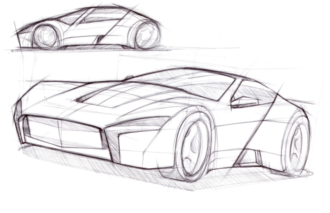
We are all guilty of it. Every tech team wants to show off their stack as this big beautiful Ferrari they are proud of. What they often omit is what is glued together by duct tape and 20 other cars they built without engines.
I think this is disparaging to new data scientists. Creating these things is full of false starts and often you end up not where you intended to go, but a good enough direction. They need to see where experts fail, and where they prioritize a must have vs nice to have. Let’s get our hands dirty.
RTR tech is World class. This is going to be the story of how this team will be able to deliver that Ferrari in a month! I hope this gives you insight on how to build things in practice and take away some practical wisdom for that Lamborghini you are going to build.
Backstory
It was a couple of weeks ago that I was sitting in a room with Anushka (GM of Unlimited, our membership program), Vijay (Chief Data Officer, my boss) and Arielle (Director of Product Management, putting it all together). We had a singular goal – how to make product discovery for Unlimited faster. The current recommendations had served us well, but we now need new UX and algos to make this happen. We had learnt from surveys and churn analysis that this is the right thing to work on. But we were short on time from when we start. We had to have a recommendation engine in a month.
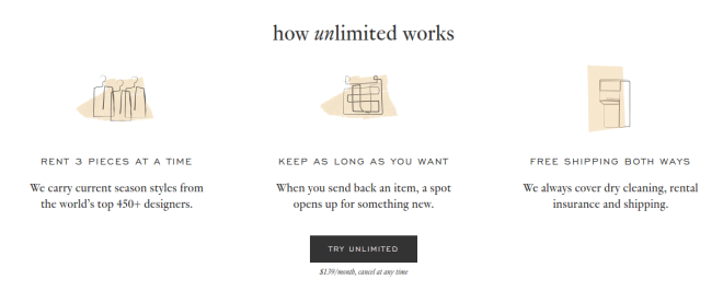
Unlimited is your subscription to Fashion. Members pay $139 a month for 3 items at a time. They can hold it for as long as they want. They can return them and get new ones, or buy them. The biggest selling point is our amazing inventory. We have a breadth of designer styles at high price points. So you can dress like a millionaire on a budget.
At high level, we want carousels of products, that are appropriate for that user’s style and fit, a la Netflix, Spotify. We want this to update online (current one is offline) and give recommendations to new users when they start. We want different sorts of carousels – ones made by the algorithms showcasing their styles, vs sorting others by our stylists. And still others saying “because you like X”.
This is naturally impossible in this timeline. However, I did build the first recommendation engine for RTR from the ground up all five years ago. I had also built the current recos for Unlimited when the program was new. We had a lot more existing pipelines and resources I could use. Plus I was getting help this time around, Sean, a bright young analyst who wants to get into Machine Learning.
This is the reality of startups. You can spend a lot of time getting something prioritized on the roadmap, and when it is, it’s a short window. And you can’t miss.
So we aren’t going to miss. And to keep me honest, I’m going to try to write about the process here. Fair warning, I’m not a habitual blogger and doing this after a full day of work, so we will see if this lasts.
What we have:
- Offline recos computed by a scala job
- Pixels (messages) coming back with what the user actually did
- MPP Data warehouse that can process pixels, orders, views, etc
- Serving pre-computed recos via a reco engine that is basically a giant cache. It serves user->products, user->events, event->products, products->products. All models pre-computed offline.
- An AI platform I built to understand images, called DeepDress, powering some products
- Lots of models from my previous research regarding our recommendations
We now have to deliver online recos, and by carousel.
My plan of attack:
- Reuse things we have built before
- Make the end-to-end pipe (data -> algo -> validation -> serving -> data)
- Make sure validation framework is in place, we need to know which metric correlates to outcome we really want to measure (churn).
- Keep it simple, we need a baseline we can improve on. Ideally two algorithms to compare.
- Allow for misses. Things aren’t going to be perfect, account for them up-front.
- Make sure Sean learns something tangible here that gets him excited about doing more things, not overwhelmed.
- Make sure any shortcuts are documented with TODOs and MEHs. We need to know where the duct tape is in context.
Let’s break it down into tracks – engineering, data science, design/product.
The engineering architecture
Before we agree on what to build, we need to agree on what success from the Engineering metrics looks like. So I proposed the following engineering metrics,
- Things will go wrong, we need safety valves:
- Code breaks – Uptime SLA (say 90%), should have fallbacks.
- Latency SLA:
- computation takes longer than say 200ms so we have to return something to the user.
- New recos reflect the actions taken by the user, in say less than 30 minutes. This means that recos should reflect actions taken by users at most 30 minutes ago.
- Flexible: We don’t know what model will work. We will change this often and experiment.
- Scaling: We need to be able to scale horizontally. This pipe should eventually replace our Classic (regular recos) pipe.
- Separation of concerns: What does Data Science do, what does Engineering do
- Language used: Engineering uses JAVA for all backend services. I have used C++ (wrapped in R) in the past, JAVA for another solver for fulfillment, scala for refactor of personalization with Anthony (who is now at Google).
Our simple proposal based on all this at the time is to create a scala library that we use to create the model. And the same library can used by the online portion at Engineering writes to load and predict from the model. This is the path of least resistance because JVM allows them to call it seamlessly, and we already have offline recommendations being computed by a Bayesian model written in scala.
The big thing here is that the JAVA portion (owned by Engineering) will have multiple fallbacks. For every type of recommendation, it can go to a set of carousels and products it can deliver. Strictly speaking, Data science ML library is research and the code to serve them is Engineering. If the ML library throws an exception, the engineering portion should know what to do about it (go to previous version of model, etc).
The other is scaling, each online serving shard only needs to know about a subset of users. We will use LSH tricks for this.
Here is the cartoon version of what we jointly proposed:
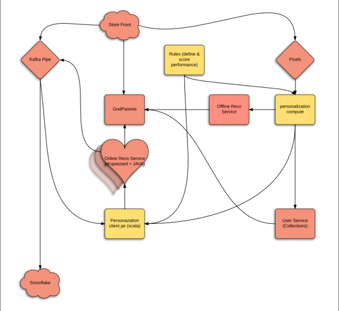
The yellow parts are new as well as the heart.
Being a software architect in early 00s makes me believe that I can still do it. However, I’m frequently wrong. Luckily John (Director of Engineering) and Jade (Director of Platoform services) took it over and rescued the drowning baby. They thought of all the edge cases and we made a lot of decisions on what we can and cannot do for MVP. Jay (Director of ETL) took over the pipeline cartoon drawing here and came up with a robust proposal that actually works with our new data warehouse – Snowflake.
The pink parts are owned by Engineering and yellow by Data Science.
OK, we have very rough edges for engineering. John is spearheading this. He broke it down with Engineering Leads (Rod and Devin) and the deeply talented engineering team (Christine, August, Denitza, Jon and Kaixi). He has all the way from user stories down to actual API requirements that MLLib needs to respond to. We also have an open question on language for the MLLib, so we are trying to get consensus.
But this seems possible to do in three sprints given the talent we have. Each sprint is 2 weeks, which is 10 working days each. So yeah, 30 days*.
This is parallel to the algorithms and design tracks. We will talk about that tomorrow.
Off to the races…
P.S got delayed posting this (today is Thursday, not Monday), but will try to keep the timeline.
PPS. Does the above sound interesting? Come work with us
<featured image via here>
Dreaming up new dresses via AI and game theory
Level: Beginner, circa 2014
Or I can haz fashion.
Here are some pretty pictures to motivate you

These are all ‘dreamt’ by a neural net. OK, now for the old bait and switch. Let’s talk Deep Learning for a second.
For the uninitiated, traditional machine learning works something like this. Say you are trying to predict housing prices using square footage. You have relevant data with those fields. So you plot the two and see if there appears to be a relationship.

Looks like there is. Usually, you start with a simple algorithm to learn that relationship. Let’s say we used linear for starters, which gets us –

price ~ 6.6 * lotsize + 34,136
Then you look at the errors, and you aren’t satisfied. Maybe this isn’t a straight line after all. Often the next thing to try is to transform the input parameters to make them look linear. So a typical transform in the above case would be natural log. Now the relationship looks like this
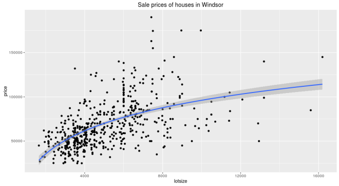
and equation
price ~ 37,660 * log(lotsize) - 250,728
And you are rewarded with better results. These sort of transforms are the bread and butter of traditional machine learning. But of course we prefer a fancier term, feature engineering.
But what are you really doing? You are transforming the input space to make the simple line fit. You still want to fit a line, but are mangling the input plane to make it go through that line. It’s like holding your breath to shimmy into a pair of jeans you have owned for longer than you should.
What if you could let the model transform the input all it needs, and build on top of the last transform one step at a time, to put the data in the right shape for your classifier? That’s exactly what deep learning does for you. And at the end, the last layer is a simple linear classifier.
This isn’t exactly a new concept, Bayesians already do this. But they don’t have a fast enough algorithm yet and the models are a bit too custom – making it hard to generalize to a new problem.
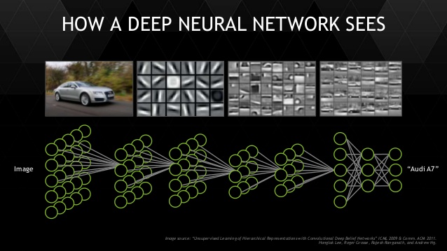
We are going to talk about dresses, so the right data format happens to be photos. To a computer, that is a matrix of numbers of height x width x 3 channels (Red, Green, Blue).
Sidenote: The above representation is not perfect. It is important to note that photo format has limitations. In real life, you don’t have borders (padding), you can move your eyes and see further. Borders are a limitation of the medium. Real vision is a fluid and complex thing (mind fills in details, nose is invisible, etc). Photos are just a good approximation of that.
Convolution transforms are designed specifically to learn from this format. It’s job is to transform the input space spatially. So lower layers do versions of edge detection, blurring, etc. And higher layers begin to understand that the combination of which edges means a collar or a sleeve. Finally, linear classifier on top as before to figure out which dress it is. As before, the model learns which convolutions to do in order to achieve the final result. It is not taught edge detection specifically but it will decide to detect a particular edge if it makes it easy for the linear classifier.
Deep learning is responsible for some impressive results. However, those impressive results require lots of data. If you aren’t so lucky, there still are a few options.
One option is transfer learning. The basic idea is that you train the network to learn to distinguish between objects on a large dataset. Then freeze the early layers and train just the last few layers very slowly on your data for it to understand how the same corners it learnt by distinguishing cats and dogs. can be used to piece together a dress.
In my experience, this tends to overfit. In other words, it doesn’t work as well for new (unseen) data. And we don’t get those advertised 90+% accuracy.
So what else can we do?
Here is a crazy idea (thanks Ian Goodfellow, 2014). Why don’t we generate our own data?
There are other data augmentation techniques (adding noise to existing input, Bayesian techniques and others) but I was looking for an excuse to generate sharp pictures of dresses anyway. So that’s what we will do.
Our net that distinguishes between classes is called a discriminator (missed opportunity to call it connoisseur). For now, we will assume all it does is say whether or not what it sees is a dress.
The idea is to invert this discriminator to generate from noise. This is called a generator. This involves inverting the convolution to a deconv layer. The loss is also negative of the Discriminator loss.
We pitch the two nets against each other but with an odd setup. In the first half of the game, we sample real data and the discriminator tries to say that this is a dress. In the second half, the generator takes in random noise and comes up with a new dress. We then sample and feed that to our discriminator that tries to say that this is not a real dress. We then back propagate the errors through the whole thing.
Over time the discriminator tries to create fakes to fool the generator. And generator tries to guard against this treachery. This goes on till they reach an equilibrium. At this point the discriminator can no longer tell real from fake dresses (50/50). Yes guys, this was the time for game theory.

We now have two nets – a much better discriminator than before because it trained on a lot more data. And a generator that can generate decent fakery.
But you ask, I thought this was ‘sane’ alytics. Where is the practical stuff!
Well, the discriminator has been fed a steady diet of fake dresses and is better at telling real from fake than when it started. It overfits less because it has trained on more data. And sure, we get the generator for free. The images in this article are from the baseline (Alexnetish) generator but theoretically using something better like Resnet should work even better.
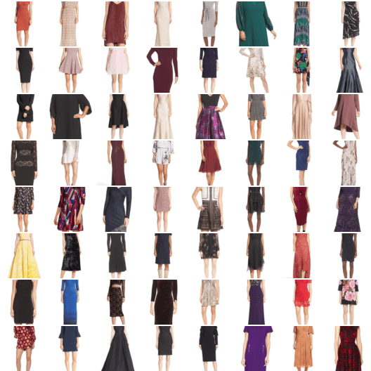
Here are some original sample pictures that we had for input
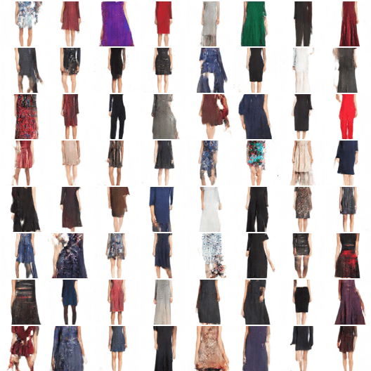
Here are some results from the generator after training.
And let’s make the distinction from adding noise to data. This is generating data from noise. See this transition to understand how it evolves over training iterations.
The discriminator learns to distinguish between this being a dress vs any fake samples. The generator plays the game and is still generating not very dress like samples at 500 iterations

And after 130,000 iterations, it can generate something like this
Here is a snippet of how it learns

While not perfect, this is impressive from two years ago when this was first introduced.
But wait, there is more. Folks have been able to generate new bedrooms, improve resolution of a photo (CSI Enhance!), make folks with RBF smile, predict what happens in the next frame of the video (compress) and generated colorful birds from text.
We don’t yet know everything GANs can do. But it is already proving to be a useful tool.
Want to generate on your own data? See DCGAN code from Facebook here and (more efficient!) WassersteinGAN here.
Want to learn more? Here is a deeper dive on different kinds of GANs.
This is a rapidly evolving field, so new papers come out all the time. We aren’t too far from dreaming up different dresses for everyone’s personal style and fit, at scale.
